Constrained routes and distributions with route_between() and predict_between()

library(BirdFlowR)
bf <- BirdFlowModels::amewoo

route_between() samples synthetic migration routes conditioned on observed locations at specific times. predict_between() computes the smooth posterior marginal distribution at every timestep given the same observations. Both functions use a Hidden Markov Model approach: a forward filter followed by backward sampling (routes) or a backward filter and forward-backward combination (distributions).

---

route_between()

Two hard observations

The most common use case: a bird banded at a wintering site and recaptured at a breeding site. We specify the two locations as lat/lon and convert to the model’s CRS.

# Known locations in WGS84 lat/lon
# (e.g. banding release in Louisiana, recapture in Maine)
lon <- c(-91.5, -68.5)
lat <- c(30.5,  45.5)

# Convert to model CRS
xy <- latlon_to_xy(lat = lat, lon = lon, bf)

rts <- route_between(bf, n = 20,
                     x_coord = xy$x,
                     y_coord = xy$y,
                     date    = c("2023-02-15", "2023-05-01"))

plot_routes(rts)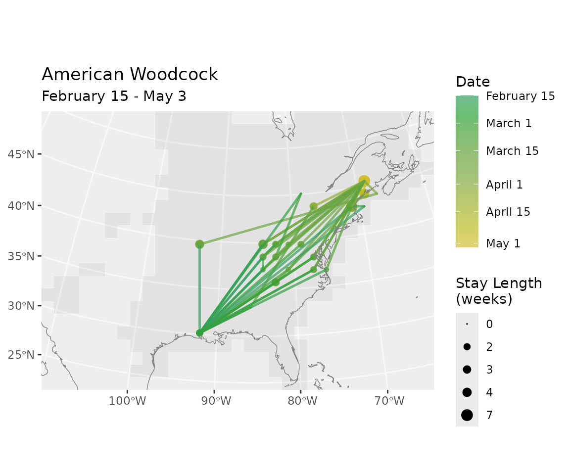

Compare with unconstrained routes

Route the same time period with route() to see what unconstrained migration looks like for this species.

rts_free <- route(bf, n = 20,
                  start = "2023-02-15",
                  end   = "2023-05-01")

plot_routes(rts_free)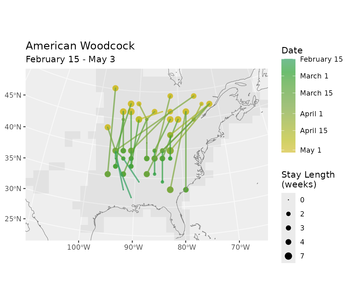

Several intermediate observations

Three observations along a migration path, as if from multiple resightings.

lon <- c(-91.5, -85.0, -78.0, -68.5)
lat <- c( 30.5,  35.0,  40.0,  45.5)
dates <- c("2023-02-15", "2023-03-15", "2023-04-10", "2023-05-01")

xy <- latlon_to_xy(lat = lat, lon = lon, bf)

rts_multi <- route_between(bf, n = 20,
                           x_coord = xy$x,
                           y_coord = xy$y,
                           date    = dates)

plot_routes(rts_multi)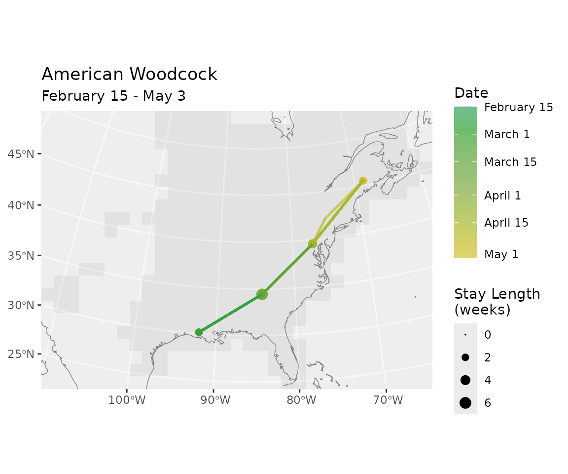

Soft observations (potentials)

Here we simulate three geolocator-style likelihood surfaces: broad Gaussian blobs centered on known locations, representing uncertain position estimates.

# Helper: Gaussian potential centered on a cell closest to (lon0, lat0)
make_gaussian_potential <- function(lon0, lat0, sigma_km, bf) {
  xy0 <- latlon_to_xy(lat = lat0, lon = lon0, bf)
  all_xy <- i_to_xy(seq_len(n_active(bf)), bf)
  dist_m <- sqrt((all_xy$x - xy0$x)^2 + (all_xy$y - xy0$y)^2)
  phi <- exp(-0.5 * (dist_m / (sigma_km * 1000))^2)
  phi
}

# Three rough position estimates (sigma = 300 km)
lons  <- c(-91.5, -82.0, -68.5)
lats  <- c( 30.5,  38.0,  45.5)
dates <- c("2023-02-15", "2023-04-01", "2023-05-01")
sigma <- 300

obs_matrix <- sapply(seq_along(lons), function(k) {
  make_gaussian_potential(lons[k], lats[k], sigma, bf)
})
colnames(obs_matrix) <- paste0("t", lookup_timestep(dates, bf))

rts_soft <- route_between(bf, n = 20, potentials = obs_matrix)

plot_routes(rts_soft)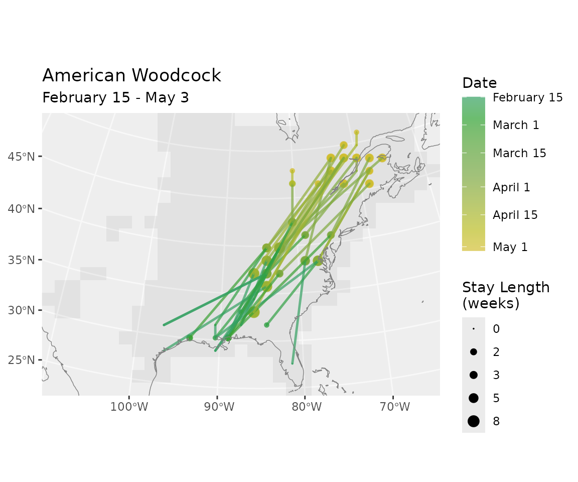

---

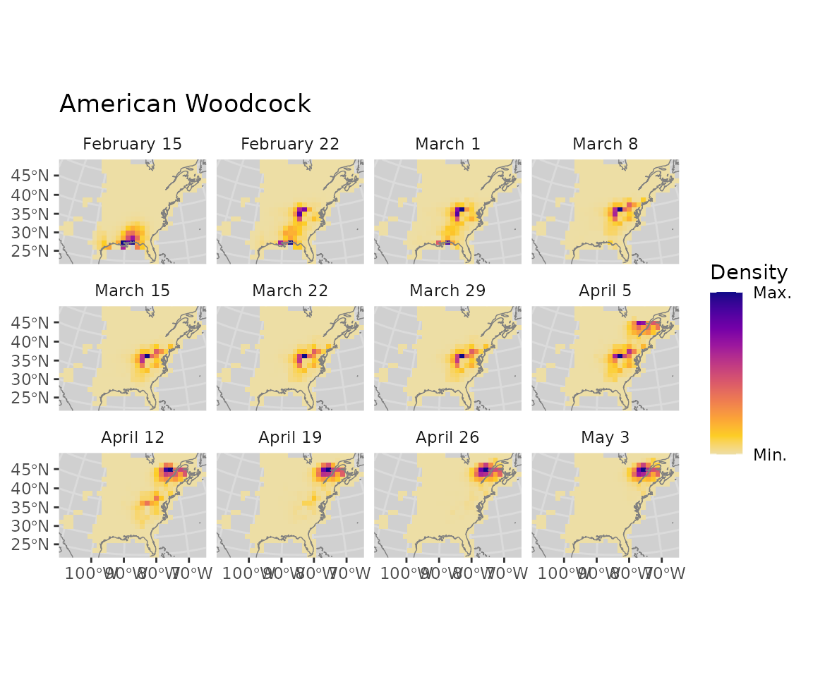
predict_between()

predict_between() returns the marginal probability distribution at every timestep conditioned on the observations — the smooth posterior over location, rather than sampled routes.

Two hard observations

The same two endpoints as above, but instead of routes we get a probability surface at each timestep.

xy <- latlon_to_xy(lat = c(30.5, 45.5), lon = c(-91.5, -68.5), bf)

distr <- predict_between(bf,
                         x_coord = xy$x,
                         y_coord = xy$y,
                         date    = c("2023-02-15", "2023-05-01"))

cat("Dimensions:", dim(distr), "\n")
#> Dimensions: 342 12
cat("Log-likelihood of observations:", round(attr(distr, "log_z"), 2), "\n")
#> Log-likelihood of observations: -7.36

plot_distr(distr, bf, dynamic_scale = TRUE)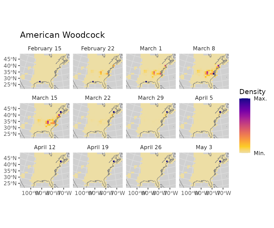

Compare: unconstrained vs constrained marginals

predict() gives the unconstrained forward distribution from the start location. predict_between() additionally pulls the distribution back toward the known end location.

distr_start <- distr[, 1]  # one-hot at the start cell
distr_free  <- predict(bf, distr_start,
                       start = "2023-02-15", end = "2023-05-01")

# Show the middle timestep from each
mid <- ncol(distr) %/% 2
both <- cbind(distr_free[, mid], distr[, mid])
colnames(both) <- c("Unconstrained (predict)", "Constrained (predict_between)")
plot_distr(both, bf, dynamic_scale = TRUE)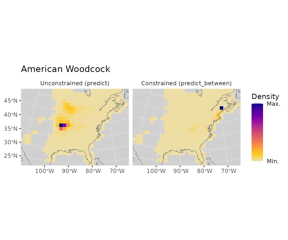

Several intermediate observations

With multiple pinned locations, the marginals are squeezed toward each observation at the relevant timestep.

lon   <- c(-91.5, -85.0, -78.0, -68.5)
lat   <- c( 30.5,  35.0,  40.0,  45.5)
dates <- c("2023-02-15", "2023-03-15", "2023-04-10", "2023-05-01")

xy <- latlon_to_xy(lat = lat, lon = lon, bf)

distr_multi <- predict_between(bf,
                               x_coord = xy$x,
                               y_coord = xy$y,
                               date    = dates)

plot_distr(distr_multi, bf, dynamic_scale = TRUE)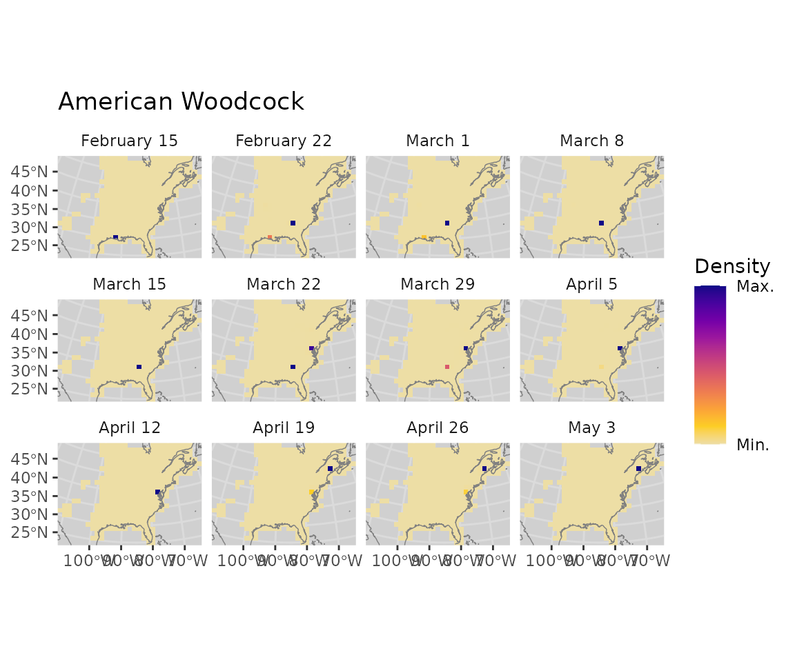

Soft observations (potentials)

The same Gaussian likelihood surfaces from the route_between() soft-obs example above, but now showing the smoothed posterior distributions rather than sampled routes.

distr_soft <- predict_between(bf, potentials = obs_matrix)

plot_distr(distr_soft, bf, dynamic_scale = TRUE)